Python: LightGBM の学習率と精度および最適なイテレーション数の関係について

勾配ブースティング決定木 (Gradient Boosting Decision Tree; GBDT) では、以下が経験則として知られている。

• 学習率 (Learning Rate) を下げることで精度が高まる
• 一方で、学習にはより多くのイテレーション数 (≒時間) を必要とする

しかしながら、上記が実際に実験などで示される機会はさほど無いように思われた。 そこで、今回は代表的な GBDT の実装のひとつである LightGBM と、疑似的に生成した学習データを使ってそれを確かめていく。 確かめる内容としては、以下のそれぞれのタスクで学習率を変化させながら精度と最適なイテレーション数の関係を記録して可視化する。

• 二値分類タスク
• 多値分類タスク
• 回帰タスク

使った環境は次のとおり。

$ sw_vers
ProductName:    macOS
ProductVersion: 12.6.2
BuildVersion:   21G320
$ uname -srm
Darwin 21.6.0 arm64
$ python -V           
Python 3.10.9
$ python -m pip list | egrep "(lightgbm|scikit-learn|matplotlib)"
lightgbm          3.3.4
matplotlib        3.6.2
scikit-learn      1.2.0

もくじ

下準備

あらかじめ、必要なパッケージをインストールしておく。

$ pip install lightgbm scikit-learn matplotlib

二値分類タスク

まずは二値分類タスクから。 早速、以下にサンプルコードを示す。 サンプルコードでは、擬似的な学習データを scikit-learn で生成して、それを LightGBM で学習し交差検証している。 最適なイテレーション数については Early Stopping を使ってメトリックが平均的に改善しなくなったタイミングを記録する。 損失関数とメトリックには、いずれも LogLoss を使っている。

import logging

import lightgbm as lgb
from sklearn.datasets import make_classification
from sklearn.model_selection import StratifiedKFold
from matplotlib import pyplot as plt


def main():
    logging.basicConfig(level=logging.INFO)

    # 疑似的な学習データを作るためのパラメータ
    args = {
        # データ点数
        "n_samples": 100_000,
        # 次元数
        "n_features": 100,
        # その中で意味のあるもの
        "n_informative": 10,
        # 重複や繰り返しはなし
        "n_redundant": 0,
        "n_repeated": 0,
        # 二値分類問題
        "n_classes": 2,
        # 生成に用いる乱数
        "random_state": 42,
        # 特徴の順序をシャッフルしない (先頭の次元が informative になる)
        "shuffle": False,
    }
    x, y = make_classification(**args)

    # StratifiedKFold で交差検証する
    folds = StratifiedKFold(
        n_splits=5,
        shuffle=True,
        random_state=42,
    )

    lgb_train = lgb.Dataset(x, y)
    lgb_params = {
        "objective": "binary",
        "metric": "binary_logloss",
        "seed": 42,
        "deterministic": True,
        "verbose": -1,
    }

    # 学習率を変化させながら精度と最適なイテレーション数を記録する
    best_iterations = {}
    best_performances = {}
    for lr in [0.8, 0.4, 0.2, 0.1, 0.05, 0.025, 0.0125]:
        lgb_params["learning_rate"] = lr
        callbacks = [
            lgb.log_evaluation(
                period=100,
                show_stdv=True,
            ),
            lgb.early_stopping(
                stopping_rounds=10_000,
                first_metric_only=True,
            ),
        ]
        cv_result = lgb.cv(
            params=lgb_params,
            train_set=lgb_train,
            num_boost_round=1_000_000,
            callbacks=callbacks,
            folds=folds,
            return_cvbooster=True,
        )
        best_iteration = cv_result["cvbooster"].best_iteration
        best_iterations[lr] = best_iteration
        logging.info("best iteration (lr: %f): %d", lr, best_iteration)

        best_performance = cv_result[f"{lgb_params['metric']}-mean"][-1]
        best_performances[lr] = best_performance
        logging.info("best performance (lr: %f): %.6f", lr, best_performance)

    # 結果を 2 軸グラフで可視化する
    fig, ax1 = plt.subplots(1, 1)
    ax1.plot(
        list(best_iterations.keys()),
        list(best_iterations.values()),
        marker="o",
        color="r",
        label="iterations",
    )
    ax1.set_xlabel("learning rate")
    ax1.set_ylabel("best iteration")
    ax1.set_title(f"objective: {lgb_params['objective']}")
    ax2 = ax1.twinx()
    ax2.plot(
        list(best_performances.keys()),
        list(best_performances.values()),
        marker="+",
        color="b",
        label="performances",
    )
    ax2.set_ylabel("best performance")

    axes = [ax1, ax2]
    ax1.legend(
        [ax.get_legend_handles_labels()[0][0] for ax in axes],
        [ax.get_legend_handles_labels()[1][0] for ax in axes],
    )
    fig.savefig(f"{lgb_params['objective']}.png")

    logging.info("best iterations: %s", best_iterations)
    logging.info("best performances: %s", best_performances)


if __name__ == "__main__":
    main()

上記を実行する。 実際に実行すると、それなりに時間がかかるので気長に待つ。

$ python binary.py

... (省略) ...

INFO:root:best iterations: {0.8: 10, 0.4: 24, 0.2: 226, 0.1: 443, 0.05: 950, 0.025: 1832, 0.0125: 3848}
INFO:root:best performances: {0.8: 0.09831524322108712, 0.4: 0.0828017991689846, 0.2: 0.06952118448905203, 0.1: 0.06681424674263811, 0.05: 0.06607646242537414, 0.025: 0.06574445115864827, 0.0125: 0.06539702674132752}

実行が完了すると、以下のようなグラフが得られる。 横軸が学習率で、縦軸が精度 (右) と最適なイテレーション数 (左) になっている。

二値分類タスクにおける関係性

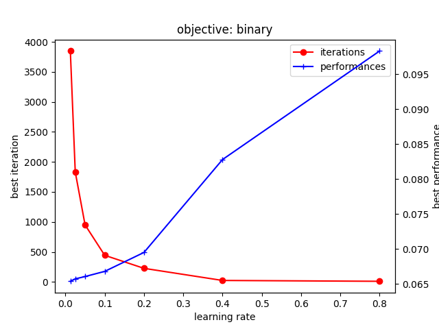
上記から、学習率を下げることで精度が改善する一方、最適なイテレーション数は増加することが確認できる。 とくに、学習率が小さくなると、急激に増加するイテレーション数と比較して精度の向上する幅は小さい。 なお、イテレーション数はニアリーイコールで学習にかかる時間と見なすこともできる。 つまり、ごくわずかな精度の向上を得るために、より多くの学習時間を要することになる。

多値分類タスク

続いては多値分類タスクで確認する。 ただし、変わっているのは生成するデータと LightGBM の学習パラメータが多値分類用のものになったところだけ。 損失とメトリックには、いずれも Softmax を用いる。

import logging

import lightgbm as lgb
from sklearn.datasets import make_classification
from sklearn.model_selection import StratifiedKFold
from matplotlib import pyplot as plt


def main():
    logging.basicConfig(level=logging.INFO)

    args = {
        "n_samples": 100_000,
        "n_features": 100,
        "n_informative": 10,
        "n_redundant": 0,
        "n_repeated": 0,
        # 多値分類問題 (5 クラス)
        "n_classes": 5,
        "random_state": 42,
        "shuffle": False,
    }
    x, y = make_classification(**args)

    folds = StratifiedKFold(
        n_splits=5,
        shuffle=True,
        random_state=42,
    )

    lgb_train = lgb.Dataset(x, y)
    lgb_params = {
        "objective": "multiclass",
        "num_class": 5,
        "metric": "multi_logloss",
        "seed": 42,
        "deterministic": True,
        "verbose": -1,
    }

    best_iterations = {}
    best_performances = {}
    for lr in [0.8, 0.4, 0.2, 0.1, 0.05, 0.025, 0.0125]:
        lgb_params["learning_rate"] = lr
        callbacks = [
            lgb.log_evaluation(
                period=100,
                show_stdv=True,
            ),
            lgb.early_stopping(
                stopping_rounds=10_000,
                first_metric_only=True,
            ),
        ]
        cv_result = lgb.cv(
            params=lgb_params,
            train_set=lgb_train,
            num_boost_round=1_000_000,
            callbacks=callbacks,
            folds=folds,
            return_cvbooster=True,
        )
        best_iteration = cv_result["cvbooster"].best_iteration
        best_iterations[lr] = best_iteration
        logging.info("best iteration (lr: %f): %d", lr, best_iteration)

        best_performance = cv_result[f"{lgb_params['metric']}-mean"][-1]
        best_performances[lr] = best_performance
        logging.info("best performance (lr: %f): %.6f", lr, best_performance)

    fig, ax1 = plt.subplots(1, 1)
    ax1.plot(
        list(best_iterations.keys()),
        list(best_iterations.values()),
        marker="o",
        color="r",
        label="iterations",
    )
    ax1.set_xlabel("learning rate")
    ax1.set_ylabel("best iteration")
    ax1.set_title(f"objective: {lgb_params['objective']}")
    ax2 = ax1.twinx()
    ax2.plot(
        list(best_performances.keys()),
        list(best_performances.values()),
        marker="+",
        color="b",
        label="performances",
    )
    ax2.set_ylabel("best performance")

    axes = [ax1, ax2]
    ax1.legend(
        [ax.get_legend_handles_labels()[0][0] for ax in axes],
        [ax.get_legend_handles_labels()[1][0] for ax in axes],
    )
    fig.savefig(f"{lgb_params['objective']}.png")

    logging.info("best iterations: %s", best_iterations)
    logging.info("best performances: %s", best_performances)


if __name__ == "__main__":
    main()

上記を実行する。

$ python multiclass.py

... (省略) ...

INFO:root:best iterations: {0.8: 11, 0.4: 85, 0.2: 420, 0.1: 931, 0.05: 1853, 0.025: 3848, 0.0125: 7501}
INFO:root:best performances: {0.8: 0.477352753580447, 0.4: 0.36786071609859394, 0.2: 0.3046891483717674, 0.1: 0.29422504356417634, 0.05: 0.2910298309291036, 0.025: 0.2904041640822766, 0.0125: 0.2902090219284779}

以下のグラフが得られる。

多値分類タスクにおける関係性

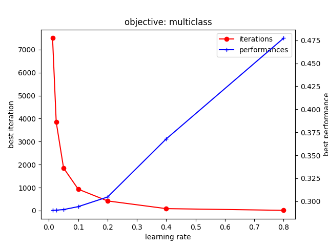
多値分類タスクについても、先ほどと概ね同じ傾向が確認できる。 LightGBM は多値分類問題を扱う際に、二値分類するブースティング決定木をクラス数分生成しているはずなので、それはそうという感じかもしれない。

回帰タスク (MSE)

続いては回帰タスクを確認する。 データは回帰タスク用になっており、交差検証は単純な Random KFold で実施する。 損失とメトリックには、いずれも MSE (Mean Squared Error) を使っている。

import logging

import lightgbm as lgb
from sklearn.datasets import make_regression
from sklearn.model_selection import KFold
from matplotlib import pyplot as plt


def main():
    logging.basicConfig(level=logging.INFO)

    # 回帰タスク用の疑似データを生成する
    args = {
        "n_samples": 100_000,
        "n_features": 100,
        "n_informative": 10,
        "random_state": 42,
        "shuffle": False,
    }
    x, y = make_regression(**args)

    # 単純な Random KFold で検証する
    folds = KFold(
        n_splits=5,
        shuffle=True,
        random_state=42,
    )

    lgb_train = lgb.Dataset(x, y)
    lgb_params = {
        "objective": "l1",
        "metric": "l1",
        "seed": 42,
        "deterministic": True,
        "verbose": -1,
    }

    best_iterations = {}
    best_performances = {}
    for lr in [0.8, 0.4, 0.2, 0.1, 0.05, 0.025, 0.0125]:
        lgb_params["learning_rate"] = lr
        callbacks = [
            lgb.log_evaluation(
                period=100,
                show_stdv=True,
            ),
            lgb.early_stopping(
                stopping_rounds=10_000,
                first_metric_only=True,
            ),
        ]
        cv_result = lgb.cv(
            params=lgb_params,
            train_set=lgb_train,
            num_boost_round=1_000_000,
            callbacks=callbacks,
            folds=folds,
            return_cvbooster=True,
        )
        best_iteration = cv_result["cvbooster"].best_iteration
        best_iterations[lr] = best_iteration
        logging.info("best iteration (lr: %f): %d", lr, best_iteration)

        best_performance = cv_result[f"{lgb_params['metric']}-mean"][-1]
        best_performances[lr] = best_performance
        logging.info("best performance (lr: %f): %.6f", lr, best_performance)

    fig, ax1 = plt.subplots(1, 1)
    ax1.plot(
        list(best_iterations.keys()),
        list(best_iterations.values()),
        marker="o",
        color="r",
        label="iterations",
    )
    ax1.set_xlabel("learning rate")
    ax1.set_ylabel("best iteration")
    ax1.set_title(f"objective: {lgb_params['objective']}")
    ax2 = ax1.twinx()
    ax2.plot(
        list(best_performances.keys()),
        list(best_performances.values()),
        marker="+",
        color="b",
        label="performances",
    )
    ax2.set_ylabel("best performance")

    axes = [ax1, ax2]
    ax1.legend(
        [ax.get_legend_handles_labels()[0][0] for ax in axes],
        [ax.get_legend_handles_labels()[1][0] for ax in axes],
    )
    fig.savefig(f"{lgb_params['objective']}.png")

    logging.info("best iterations: %s", best_iterations)
    logging.info("best performances: %s", best_performances)


if __name__ == "__main__":
    main()

上記を実行する。

$ python l2.py

... (省略) ...

INFO:root:best iterations: {0.8: 120, 0.4: 459, 0.2: 1358, 0.1: 8218, 0.05: 18254, 0.025: 58758, 0.0125: 174082}
INFO:root:best performances: {0.8: 620.5233864841325, 0.4: 403.4180953244528, 0.2: 276.98699934231274, 0.1: 168.65622625748594, 0.05: 107.56471173868105, 0.025: 78.86550385866083, 0.0125: 66.78599993592725}

以下のグラフが得られる。

回帰タスク (MSE) の関係性

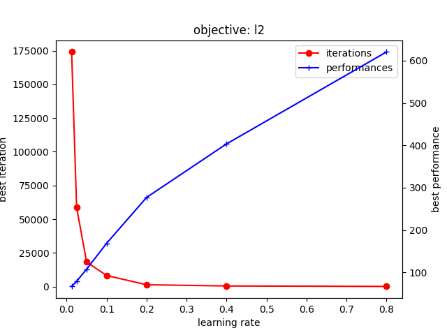
こちらも、これまでと同様の傾向が確認できる。 ただし、学習率が小さい場合のイテレーション数の増加は二値分類や多値分類に比べてより急峻になっている。

回帰タスク (MAE)

回帰タスクについては損失やメトリックも色々とあるので、一応 MAE (Mean Absolute Error) についても確認しておく。 変更点は損失とメトリックが変更されているところだけ。

import logging

import lightgbm as lgb
from sklearn.datasets import make_regression
from sklearn.model_selection import KFold
from matplotlib import pyplot as plt


def main():
    logging.basicConfig(level=logging.INFO)

    args = {
        "n_samples": 100_000,
        "n_features": 100,
        "n_informative": 10,
        "random_state": 42,
        "shuffle": False,
    }
    x, y = make_regression(**args)

    folds = KFold(
        n_splits=5,
        shuffle=True,
        random_state=42,
    )

    lgb_train = lgb.Dataset(x, y)
    lgb_params = {
        "objective": "l1",
        "metric": "l1",
        "seed": 42,
        "deterministic": True,
        "verbose": -1,
    }

    best_iterations = {}
    best_performances = {}
    for lr in [0.8, 0.4, 0.2, 0.1, 0.05, 0.025, 0.0125]:
        lgb_params["learning_rate"] = lr
        callbacks = [
            lgb.log_evaluation(
                period=100,
                show_stdv=True,
            ),
            lgb.early_stopping(
                stopping_rounds=10_000,
                first_metric_only=True,
            ),
        ]
        cv_result = lgb.cv(
            params=lgb_params,
            train_set=lgb_train,
            num_boost_round=1_000_000,
            callbacks=callbacks,
            folds=folds,
            return_cvbooster=True,
        )
        best_iteration = cv_result["cvbooster"].best_iteration
        best_iterations[lr] = best_iteration
        logging.info("best iteration (lr: %f): %d", lr, best_iteration)

        best_performance = cv_result[f"{lgb_params['metric']}-mean"][-1]
        best_performances[lr] = best_performance
        logging.info("best performance (lr: %f): %.6f", lr, best_performance)

    fig, ax1 = plt.subplots(1, 1)
    ax1.plot(
        list(best_iterations.keys()),
        list(best_iterations.values()),
        marker="o",
        color="r",
        label="iterations",
    )
    ax1.set_xlabel("learning rate")
    ax1.set_ylabel("best iteration")
    ax1.set_title(f"objective: {lgb_params['objective']}")
    ax2 = ax1.twinx()
    ax2.plot(
        list(best_performances.keys()),
        list(best_performances.values()),
        marker="+",
        color="b",
        label="performances",
    )
    ax2.set_ylabel("best performance")

    axes = [ax1, ax2]
    ax1.legend(
        [ax.get_legend_handles_labels()[0][0] for ax in axes],
        [ax.get_legend_handles_labels()[1][0] for ax in axes],
    )
    fig.savefig(f"{lgb_params['objective']}.png")

    logging.info("best iterations: %s", best_iterations)
    logging.info("best performances: %s", best_performances)


if __name__ == "__main__":
    main()

上記を実行する。

$ python l1.py

... (省略) ...

INFO:root:best iterations: {0.8: 105, 0.4: 29015, 0.2: 251095, 0.1: 349269, 0.05: 999746, 0.025: 999900, 0.0125: 999996}
INFO:root:best performances: {0.8: 24.84506083319512, 0.4: 18.973220015575627, 0.2: 14.361268813657691, 0.1: 10.862815071557257, 0.05: 8.626113874984942, 0.025: 7.535406392204019, 0.0125: 7.066955421845141}

以下のグラフが得られる。

回帰タスク (MAE) の関係性

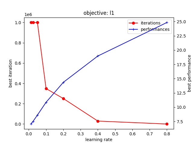
こちらも学習率を下げることで精度が改善する傾向にあることが確認できる。 ただし、MAE では MSE よりもさらに多くのイテレーション数を必要とするようだ。 とくに 0.1 未満の学習率では、あらかじめ設定したイテレーション数の上限 (1M) に達してしまっている。 とはいえ、これ以上のイテレーション数を求めると学習に時間がかかりすぎるため上限は増やさないことにした。

前述したとおり 0.1 未満の学習率ではイテレーション数の上限に達しているため、同じイテレーション数になっている。 にも関わらず、学習率が小さいほど精度が改善している点は印象的に感じる。 なぜなら、学習率が小さいと一般に学習が進むペースも遅くなることから、未学習となって精度が低くなってもおかしくないため。 この点は、Early Stopping がかからないようなごく僅かな改善は続いているものの、学習曲線的にはすでに底に到達しているためかもしれない。 MAE は他の損失関数と比較してゼロ近辺において大きな損失を生むため、そのような振る舞いになっている可能性はある。

上記を、実際に確認してみよう。 以下のサンプルコードでは、学習率が 0.0250 と 0.0125 の場合で学習曲線を比較している。 具体的には、交差検証において Out-of-Fold なデータに対する平均的なメトリックをイテレーション毎にプロットする。 先ほどの仮説が正しければ Early Stopping を引き起こさないまでも、それ以前のイテレーションにおいてメトリックはほとんど底を打っているはず。

import logging

import lightgbm as lgb
from sklearn.datasets import make_regression
from sklearn.model_selection import KFold
from matplotlib import pyplot as plt


def main():
    logging.basicConfig(level=logging.INFO)

    args = {
        "n_samples": 100_000,
        "n_features": 100,
        "n_informative": 10,
        "random_state": 42,
        "shuffle": False,
    }
    x, y = make_regression(**args)

    folds = KFold(
        n_splits=5,
        shuffle=True,
        random_state=42,
    )

    lgb_train = lgb.Dataset(x, y)
    lgb_params = {
        "objective": "l1",
        "metric": "l1",
        "seed": 42,
        "deterministic": True,
        "verbose": -1,
    }

    fig, ax1 = plt.subplots(1, 1)
    for lr in [0.025, 0.0125]:
        lgb_params["learning_rate"] = lr
        callbacks = [
            lgb.log_evaluation(
                period=1_000,
                show_stdv=True,
            ),
        ]
        cv_result = lgb.cv(
            params=lgb_params,
            train_set=lgb_train,
            num_boost_round=200_000,
            callbacks=callbacks,
            folds=folds,
            return_cvbooster=True,
        )
        eval_performances = cv_result[f"{lgb_params['metric']}-mean"]

        ax1.plot(
            [i for i, _ in enumerate(eval_performances, start=1)],
            eval_performances,
            label=f"lr: {lr:.4f}",
        )

    ax1.set_ylabel("performance")
    ax1.set_xlabel("iterations")
    ax1.legend()
    ax1.set_title(f"objective: {lgb_params['objective']}")
    fig.savefig(f"learning-curve-{lgb_params['objective']}.png")


if __name__ == "__main__":
    main()

上記を実行する。

$ learningcurve.py
...(省略)...

以下のグラフが得られる。

回帰タスク (MAE) の学習曲線 (lr: 0.0250, 0.0125)

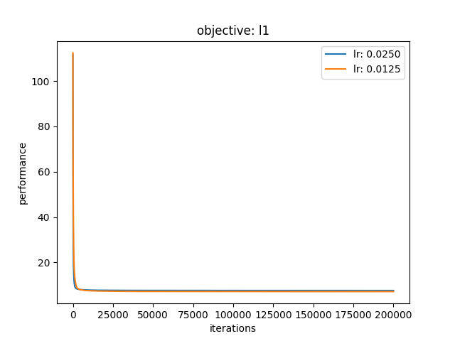
やはり、メトリックは早々に底を打っており、それ以降はダラダラとごく僅かな改善が続いているようだ。 このように明確な過学習をなかなか起こさない状況では既存の Early Stopping が有効に働かない。 そのため「メトリックが悪化したら」ではなく「改善幅が十分に小さくなったら」学習を打ち切るような Early Stopping が必要かもしれない。

まとめ

今回は、勾配ブースティング決定木について経験則として知られている以下について LightGBM を使った実験で確かめた。

• 学習率 (Learning Rate) を下げることで精度が高まる
• 一方で、学習にはより多くのイテレーション数 (≒時間) を必要とする

Kaggleで勝つデータ分析の技術